Deep dive into flow models

We previously discussed how diffusions work and their differences with AR models. There is a close family of deep learning paradigms closer to diffusions called flow models. Flow models, instead of relying on Stochastic Differential Equations, use Ordinary Differential Equations (we’ll cover them soon) in order to form a path from normally (Gaussian) distributed noise to the target data distribution.

Training objective

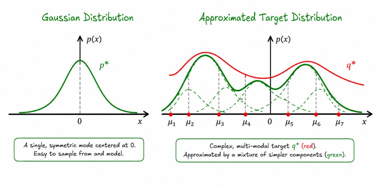
We introduce the term velocity field, which defines how the probability distribution will be moving towards the target distribution. Say, we pick an initial distribution (Gaussian) and approximate the target distribution. Then, we need to teach the model to transform the initial distribution into the target distribution. This is the main training objective that’s used both for diffusion and flow models. The major difference between them is in the techniques used to reach that goal. The illustration of our training objective is given below.

Ordinary Differential Equations

Ordinary differential equations define a condition for a trajectory, or the velocity field - 𝒗𝜽 at point x and time t:

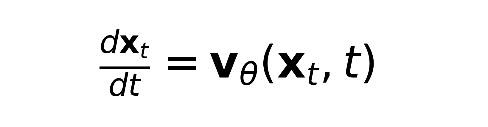
𝒗𝜽 is the neural network that we need to train, It takes the current data point and time, and outputs a velocity, pointing where and how fast to move.

Flow matching

While ODE is the core mechanism, the training objective is performed using the so-called “Flow matching” technique. Before getting to this term, let’s first define two types of vector/velocity fields:

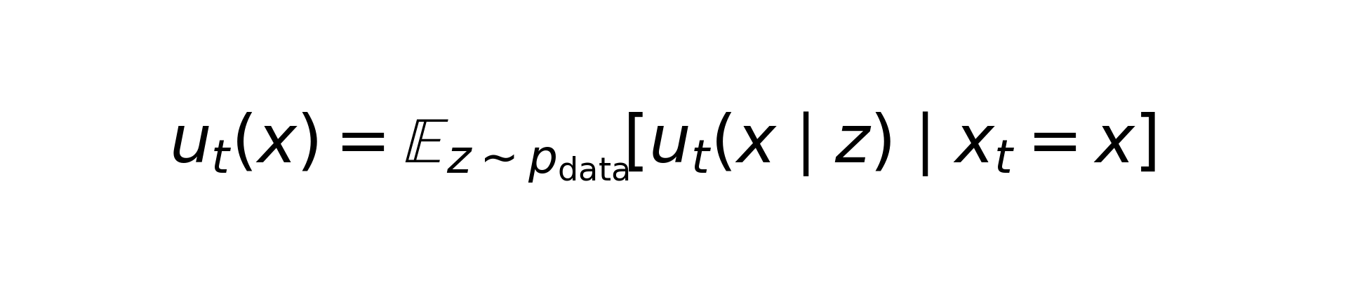
1. The marginal vector field defines the trajectory of the probability distribution by averaging conditional vector fields, weighted by how likely each data point is given xt. This is challenging because averaging over all data (as shown in the formula below) is expensive, and solving the integral of it yields an intractability.

1. The conditional vector field acts the same as marginal VF, except it samples only one data point at time t and outputs the next trajectory (vector, or you can call it a neural network), which is tractable.

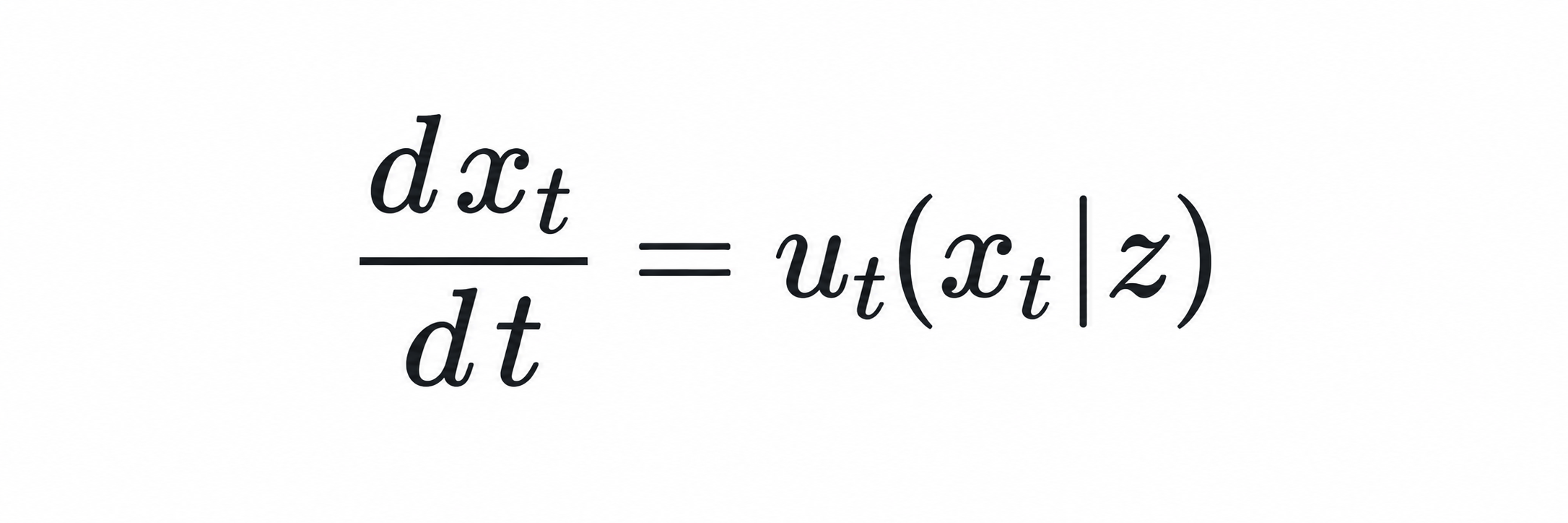
We are going to deal with Conditional VFs most of the time. Flow matching has a loss, since it regresses neural networks. The general loss function illustrates the difference between the current vector field at point x and marginal vector field at all of x points. As you might have guessed this is intractable. This is the formalized formula for Loss function of Flow Matching:

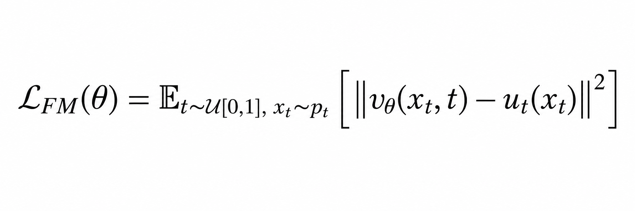
Again, we turn our attention to the simpler, yet effective loss function, called ** the conditional Flow Matching Loss**, which accounts for the difference between the current vector field and conditional vector field, which we defined above. Hence, it is tractable.

THEOREM

There is an interesting theorem which says the loss function of FM equals the conditional loss function plus some constant.

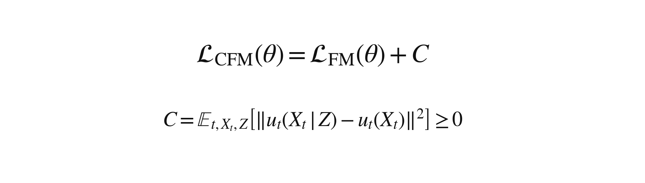
Sounds quite random, right? The key idea is that the marginal vector field is the weighted average of the conditional probabilities. And squared error of each conditional vector field adds the spread around the average, but it doesn’t depend on our parameter , hence it’s constant.

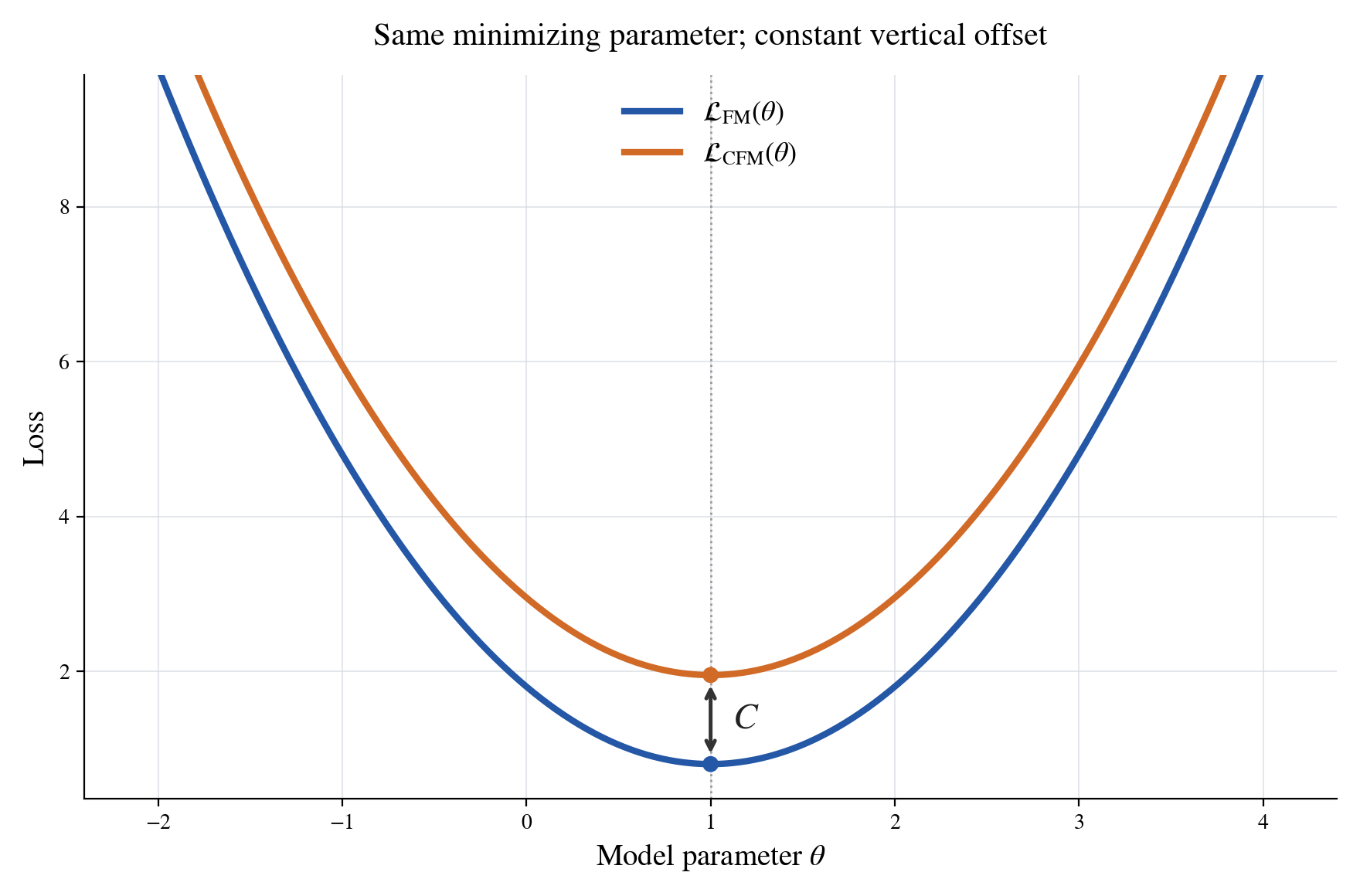
As you see, the minimum of both functions is the same; they differ only in their intercept.

So, flow matching is one of those innovative techniques that carries simplicity in its form, yet it is elegant.